Machine Learning
机器学习
与该笔记配套的代码仓库 Michel-Johnson/Machine-Learning
监督学习 (Supervised Learning)
核心思想: 从带有标签/答案的数据中学习。模型通过观察输入数据和其对应的正确输出,来学习一个映射函数,以便在未来遇到新的、未标记的输入时,能够预测出正确的输出。 Learns from being given “right answers”
-
分类 (Classification):
预测离散的类别标签。 predict categories
- 电子邮件是垃圾邮件还是非垃圾邮件?图片是猫还是狗?
-
回归 (Regression):
预测连续的数值输出。
- 预测房价、股票价格、气温。
无监督学习 (Unsupervised Learning)
核心思想: 从没有标签的数据中学习。模型不被告知正确的输出是什么,而是尝试在数据中发现隐藏的结构、模式或关系。
-
聚类 (Clustering):
将相似的数据点分组到一起,形成簇。
- 客户细分(将客户分成不同的消费群体)。
-
降维 (Dimensionality Reduction):
减少数据的特征数量,同时保留最重要的信息。
- 主成分分析 (PCA),用于数据可视化或预处理。
-
关联规则学习 (Association Rule Learning):
发现数据集中项之间的有趣关系。
- 购物篮分析(“购买了A商品的人也经常购买B商品”)。
-
异常检测 (Anomaly Detection):
识别数据集中与大多数数据显著不同的数据点(异常值或离群点)。
- 信用卡欺诈检测、网络入侵检测、设备故障预测。
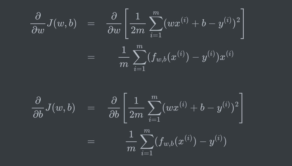
Cost function
Squared error cost fuction:
2m是为了后续求偏导后的结构好看
梯度下降 (Gradient Descent)
学习率 (Learning Rate / Step Size, 符号 或 ):
- 这是一个超参数,决定了在每次迭代中参数更新的步长大小。
- 如果学习率太小,收敛会非常缓慢。
- 如果学习率太大,可能会跳过最小值,甚至发散。
Simultaneous update
同时计算和,不然会导致计算tmp_b时的cost function偏导数时使用了更新的,可能会导致算法行为不稳定甚至发散。
Batch gradient descent 批量梯度下降
Each step of gradient descent uses all the training examples.
也就是计算偏导数时的求和从1到m都加上(使用整个训练数据集)
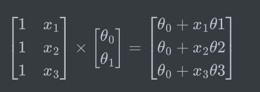
Multiple features
Normal Equation
是线性回归中求解最优参数的闭式解方法,通过最小化损失函数(如均方误差)直接得出模型参数。其核心公式
该方程通过求解下面的方程来找出使 cost function最小的参数
要求 可逆(满秩矩阵)。若不可逆(如存在多重共线性),需使用正则化或伪逆(如 numpy.linalg.pinv)
Disadvantages:
- Doesn’t generalize to other learning algorithms
- Slow when number of features is large
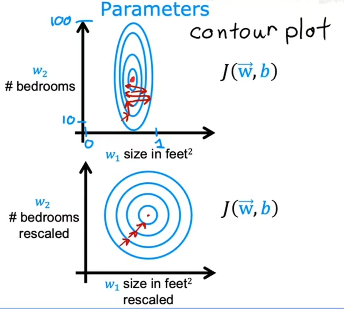
Feature Scaling
When you have different features that take on very different ranges of values, it can cause gradient descent to run slowly. But rescaling the different features so they all take on comparable range of values can speed up gradient descent significantly.
There are many ways to perform normalization:
- Mean normalization
- Z-score normalization (Standardization)
- …
This is the Wikipedia link of Feature Scaling.
Polynomial Regression
Use scikit-learn, and I wrote a piece of code using scikit-learn multivariate fitting with the help of AI.
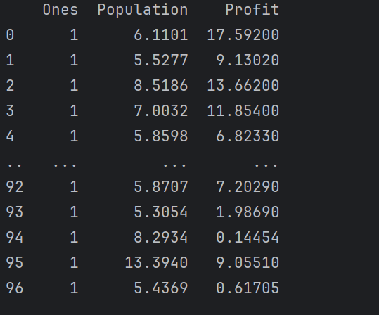
Exercise 1
- Cost function
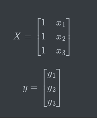
使用矩阵来计算
1 | data.insert(0, 'Ones', 1) |
加入一列,作为截距项
1 | cols = data.shape[1] # get columns of matrix , cols = 3 |
1 | theta = np.matrix(np.array([0,0])) |
被初始化为[0,0] (1*2的矩阵)
即为 X @ theta.T
1 | def computeCost(X, y, theta): |
- Batch gradient descent
完整代码:
1 | def gradientDescent(X, y, theta, alpha, iters): |
**的代码是重点
1 | term = np.multiply(error, X[:, j]) |
j=0 为截距项,根据 批量梯度下降偏导公式,两个偏导数只有 项不同,而恰好 时,为b的偏导,所以直接使用w的偏导公式即可
tmp_b同
所以term 即为 $ [f_{w,b}(x{(i)})-y{(i)} ]x^{(i)}$
后续计算较为简单
变量输入:
1 | alpha = 0.01 |
图像输出
1 | x = np.linspace(data.Population.min(), data.Population.max(), 100) |
由于多变量与单变量的gradientDescent与computeCost函数相同,只有初期因此博客中略过,可从代码中学习。
Logistic Regression
Sigmoid/Logistic function:
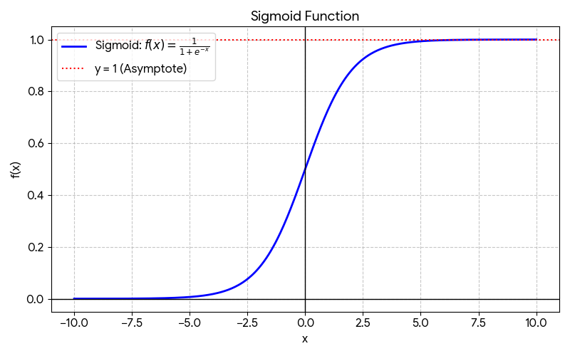
The logistic regression’s output is to think of it as outputting the probability that the class or the label y will be equal to 1 given a certain input x.
Logistic Regression:
z is not necessarily linear
With these polynomial features, you can get very complex decision boundaries.
Cost Function for Logistic Regression
The cost function gives you a way to measure how well a specific set of parameters fits the training data, and thereby gives you a way to choose better parameters.
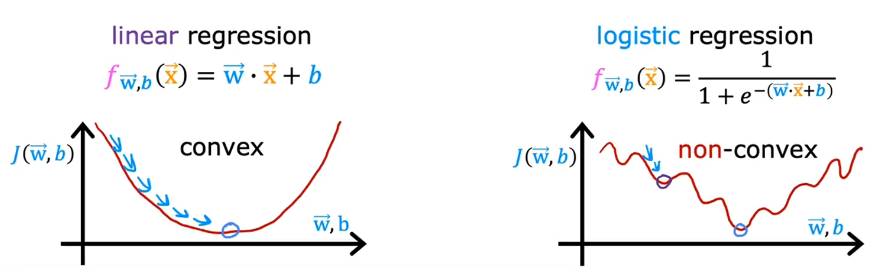
In the case of linear regression, where f of x is the linear function $f_{\vec{w},b}\left( \vec{x} \right) = \vec{w}\cdot \vec{x}+b J(\theta) = \frac{1}{2m} \sum_{i=1}^{m} ( h_\theta(x{(i)})-y{(i)} )^2$ looks like the left part. This is a convex function.
But if you try to use the same cost function for logistic regression, it will look like the right part. This becomes what’s called a non-convex cost function. It means that if you were to use the gradient descent, there are lots of local minima that you can get stuck in. So we need to use another cost function which makes the cost function convex again, so that gradient descent can be guaranteed to converge to the global minimum.
The loss function measures how well you’re doing on one training example, and it’s by summing up the losses on all of the training examples that you then get the cost function, which measures how well you’re doing on the entire training set.
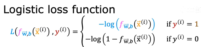
if 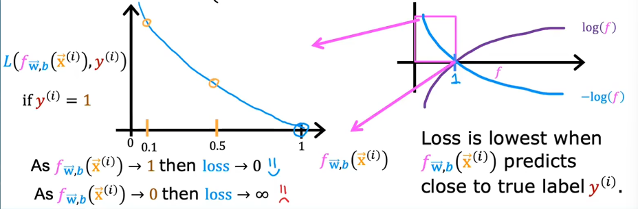
if 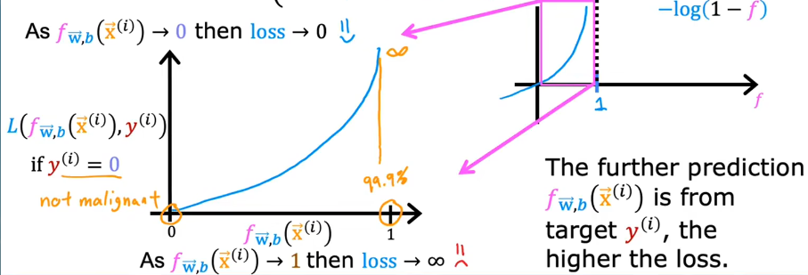
How to prove that this function is convex?..
Well, this particular cost function is derived from statistics using a statistical principle called maximum likelihood estimation, which is an idea from statistics on how to efficiently find parameters for different models.
Gradient Descent Implementation
The gradient descent algorithm is similar to the linear regression. Check it in the exercise.
The Problem of Overfitting
Bias: This occurs when the algorithm has underfit the data. It means the model cannot fit the training set well and fails to capture clear patterns present in the data.
Generalization: Make good predictions, even on brand new examples that it has never seen before.
Overfit–high variance
How to address overfitting?
- Collect more training data.
- Not use so many of these polynomial features(feature selection).
- Reduce size of parameters.(Regularization)
Cost Function with Regularization
: Regularization parameter
This new cost function trying to minimize this first term encourages the algorithm to fit the training data well by minimizing the squared differences of the predictions and the actual values. And trying to minimize the second term, the algorithm also tries to keep the parameters small, which will tend to reduce overfitting.